Pendulum ‘Q’ value and measurement methods

[John HaineParticipant @johnhaine32865]

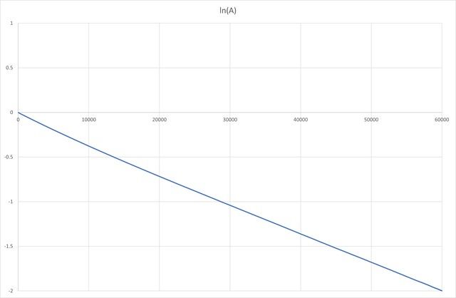
I thought that the following example of a run-down test might be useful. I took this from my new pendulum just after replacing the spring and rod. Essentially allowed the amplitude to stabilise at just above the intended operating point, then switched off the impulsing and logged amplitude as it decayed, measuring it basically by the photogate time.

The plot shows the natural log of amplitude against beat time (essentially seconds). Nearly a straight line with a barely visible "kink" after about 15000 seconds. The first part of the run (around the eventual operating point) yields a Q of about 22,500. Andrew Millington pointed out that the Q improves at lower amplitude to about 24,500. There are essentially two flow regimes around the bob it would seem, at larger amplitudes there is an increasing square-law dependence of drag on velocity whereas at lower amplitude it is essentially linear. Note that the curve is very clean with very little scatter of the points about the trend line.

[duncan webster 1Participant @duncanwebster1]

So if SOD measured Q by rundown and got the same answer as by bandwidth the argument would be resolved. I must admit some doubt over trying to measure energy loss whilst putting energy in feels problematical. Of course he might already have done this and reported it previously, my attention span isn't what it was.

[Joseph Noci 1Participant @josephnoci1]

Posted by John Haine on 16/08/2023 22:29:49:

I thought that the following example of a run-down test might be useful. I took this from my new pendulum just after replacing the spring and rod. Essentially allowed the amplitude to stabilise at just above the intended operating point, then switched off the impulsing and logged amplitude as it decayed, measuring it basically by the photogate time.

The plot shows the natural log of amplitude against beat time (essentially seconds). Nearly a straight line with a barely visible "kink" after about 15000 seconds. The first part of the run (around the eventual operating point) yields a Q of about 22,500. Andrew Millington pointed out that the Q improves at lower amplitude to about 24,500. There are essentially two flow regimes around the bob it would seem, at larger amplitudes there is an increasing square-law dependence of drag on velocity whereas at lower amplitude it is essentially linear. Note that the curve is very clean with very little scatter of the points about the trend line.

That looks nice John.

Would you refresh me please – what is your pendulum structure? – pivot style, bob ( shape, weight) rod material, and measurement method ( opto interrupter / part number)?

There are now so many topics running on pendulum, I did not manage to find your earlier descriptions and references!

[John HaineParticipant @johnhaine32865]

**LINK**

All the information in that thread Joe.

[John HaineParticipant @johnhaine32865]

Wikipedia has a good collection of information on Q. Includes a couple of useful formulae.

Time constant of decay T = 2Q/Wo where Wo = 2pi/To (To is the full period).

Then amplitude decays at A = Ao.exp(-t/To).

Setting A/Ao to various convenient values such as 0.5 or 1/e then gives the various formulas for Q in terms of number of cycles that have been quoted.

[Joseph Noci 1Participant @josephnoci1]

Posted by John Haine on 17/08/2023 07:29:04:

**LINK**

All the information in that thread Joe.

Thanks John – refreshed …

[SillyOldDufferModerator @sillyoldduffer]

Posted by SillyOldDuffer on 16/08/2023 21:15:50:

After reading SK and John's posts I decided to pour myself a couple of large sherries and go to bed early!

Dave

Last night's exciting episode ended with our hero (me because I'm writing the script) assailed on all sides. By analogy I was cuffed inside a heavily weighted crate dropped into the Atlantic north of Scapa Flow. Fortunately I'm a pulp fiction fan, where cliffhangers are resolved in the next issue with the line 'With one mighty bound he was free."

Oh well, back to the real world where I may be sunk without trace!

SK repeated my description of the bandwidth Q-factor calculation on his data and got an absurd answer. I don't think that proves the bandwidth method doesn't work. I'd like to run SK's data through my program to see what I get. If I get 198,000 too, then the clearly my approach is wrong. Any chance of making the data available via Dropbox or similar?

John Haine is more difficult to deal with because I'm well out of my depth with the maths! John said (full post above at 17:32 yesterday):

It seems to me that the resemblance of the normal distribution curve to a resonance curve is tempting but unfortunate. Assuming that Dave's period distribution is normal, its width is characterised by just one parameter, the standard deviation. The "-3dB" points are related to this but superfluous.

In practice the width of the period distribution must depend on the amplitude and noise level (i.e. the "signal to noise ratio" as well as on Q. So buried in Dave's computation is this SNR, which itself is also determined by Q (as this determines the bandwidth of the noise which is affecting the period).

In response, I didn't invent the Bandwidth method of determining Q-factor!

As I understand it Q-factor is a dimensionless indicator of the goodness of an oscillator. Any oscillator from bouncing balls to atomic clocks. To my mind a pendulum is just another oscillator following the same rules as all the others. Oscillators resonate at a particular frequency, and energy is required to keep them going. Lossy oscillators, such as a pendulum in treacle, have low Q because stirring treacle consumes lots of energy. The same pendulum swinging in a vacuum has high Q because atmospheric friction is eliminated. Exactly the same rules apply to Inductor(L) / Capacitor (C) oscillators. Although capacitors are low-loss, the inductor is a metallic wire coil and the wire is a resistor. The same inductor made of Brass wire has lower Q than one made of Copper, and Silver is better again. Energy loss in a resistive inductor behaves the same way as energy loss in a pendulum overcoming air resistance.

Two ways of measuring oscillator Q:

• Impulse the resonator once and count how many cycles it takes for the amplitude to decay by a known amount, say 50%. Q is calculated by applying a formula. This is the decay method
• Impulse the resonator to keep the resonator running continually. Amplitude peaks when the impulse frequency matches the resonant frequency. In practice the resonant frequency varies about a mean, and it has a normal distribution. When a lot of energy is needed to maintain oscillation, the resonant frequency also varies a lot – low Q. When very little energy is needed to maintain oscillation, frequency doesn't vary much. Q is calculated by determining the resonators bandwidth by getting the frequency spread by analysing a large number of periods. Narrow bandwidth means high Q, wide bandwidth means low Q. Q is calculated by applying a formula, this is the bandwidth method.

John said: 'seems to me that the resemblance of the normal distribution curve to a resonance curve is tempting but unfortunate. I disagree – I think the resonant curve of an oscillator is normally distributed unless something disturbs it. Standard Deviation isn't the whole story because, as far as I know, it doesn't describe the shape of the distribution, narrow or wide. Stdev has a dimension, whereas Q is dimensionless.

I can't argue with John's formula, but offer this from an article on the web:

This formula doesn't introduce the spectral density of the noise force component of the impulse.

Duncan suggests measuring my pendulum with both decay and bandwidth methods. Did that in the past and got a result within about 30%. Not conclusive because I didn't repeat the measurement several times. Can't do a decay measurement on my clock at the moment because it's doing a long run. For family reasons I'm short of time at present, but might find a few hours to hack a test pendulum. Alternatively, if John has decay measured one of his pendula, and has a run log, I could analyse that to see if results are similar.

Though chest deep in doubt, I still think Decay and Bandwidth are both valid ways of measuring pendulum Q.

Dave

[John HaineParticipant @johnhaine32865]

Though chest deep in doubt, I still think Decay and Bandwidth are both valid ways of measuring pendulum Q.

Absolutely they are – but I don't think your probability distribution of period is a bandwidth measure.

[SillyOldDufferModerator @sillyoldduffer]

Posted by John Haine on 17/08/2023 16:08:50:

Though chest deep in doubt, I still think Decay and Bandwidth are both valid ways of measuring pendulum Q.

Absolutely they are – but I don't think your probability distribution of period is a bandwidth measure.

OK, but what am I measuring then?

In my set-up a crystal oscillator measures the period of each beat of a pendulum, outputting a long list of similar values, standard deviation about 1mS. Averaging the list gives a value, 0.933558s, which is close to the period predicted by the usual formula from my pendulum's length. Further, plotting the distribution of periods from the list gives the bell curve expected of an oscillator.

If the peak of my bell curve gives the pendulum's correct frequency, why don't the 3dB points on the same curve give Q?

As period and frequency are equivalent, I think my data represents a spectral distribution. I'm not understanding why it's different from a resonant curve.

Gosh my head hurts!

Dave

[S KParticipant @sk20060]

Are you really using the simplistic formula from that "bandwidth of a tuned circuit" diagram? That delivers a Q of about 500, doesn't it? What formula are you actually using?

The thing is, with an S.D. of 1ms, I don't see how you can find all that much more than that with any similar bandwidth based formula. You need to focus on improving the S.D. first. If I had to guess, your measurement apparatus is probably to blame, not your pendulum.

Edited By S K on 17/08/2023 18:18:45

[SillyOldDufferModerator @sillyoldduffer]

Posted by S K on 17/08/2023 18:13:38:

Are you really using the simplistic formula from that "bandwidth of a tuned circuit" diagram? That delivers a Q of about 500, doesn't it? What formula are you actually using?

The thing is, with an S.D. of 1ms, I don't see how you can find all that much more than that with any similar bandwidth based formula. You need to focus on improving the S.D. first. If I had to guess, your measurement apparatus is probably to blame, not your pendulum.

…

I am using the 'simplistic formula' for bandwidth. As far as I know it is valid – it's in all my books! Do you have an alternative?

The diagram is from a Radio Communications Handbook, where Q= 500 is about right for an ordinary inductor/capacitor resonator at radio frequency. It doesn't represent the Q of a pendulum, quartz crystal or anything and else, just the typical shape of a resonance bell-curve.

It's how narrow the curve is at the 3dB down points that decides Q. In the example below, all three curves are of the same form but Q=1 results in a low hump, whilst Q=100 gives a sharp peak:

As I said to John in a related thread, the Q calculation I'm using reports period consistent with the physical length of my pendulum. If the calculation gets period right at the 50 percentile, why should it be wrong at 70.7 and 29.3 percentiles?

In an earlier post you said applying the bandwidth method to your pendulum gave Q=190,000. Can you share the data and calculation please, showing working. Might highlight what I'm doing wrong!

Though related there's a difference between Q and standard deviation. In my simple view Q is a measure of how much energy is needed to drive a pendulum, whilst standard deviation is a measure of the pendulums frequency stability.

I'm not too worried about by pendulum's high standard deviation because I've not found any evidence, yet, that it's related to the rate wandering. At the moment the clock is 14 seconds out in 2,835,926 which is 4.9 parts per million, so not disasterous. What's worrying me is the rate isn't altering at a steady rate, or changing with temperature or pressure. I'm letting it gather more data in hope a pattern emerges.

Dave

[S KParticipant @sk20060]

If I estimate your "half power bandwidth" to be 2 times your standard deviation (that's the number I have, anyway), then after rounding the numbers for simplicity, I get Q=1/(2*0.001)=500. How do you get over 20,000? What numbers do you have?

Also, you expressed concern about how your cumulative time error had wandered. This is due in large part to the accumulation of many small random errors in a classic random walk. If those small errors are 250 times lower (i.e., S.D. = 4us vs. 1ms), then the cumulative deviations should, in an typical run, also be 250 times lower. So yes, you do want as low a standard deviation as you can get.

Edited By S K on 18/08/2023 01:46:06

[Michael GilliganParticipant @michaelgilligan61133]

This might be useful: **LINK**

http://www.vibrationdata.com/tutorials2/half_power_bandwidth.pdf

It’s a long while since I worked in vibration testing, but it looks right.

caveat lector

MichaelG.

[John HaineParticipant @johnhaine32865]

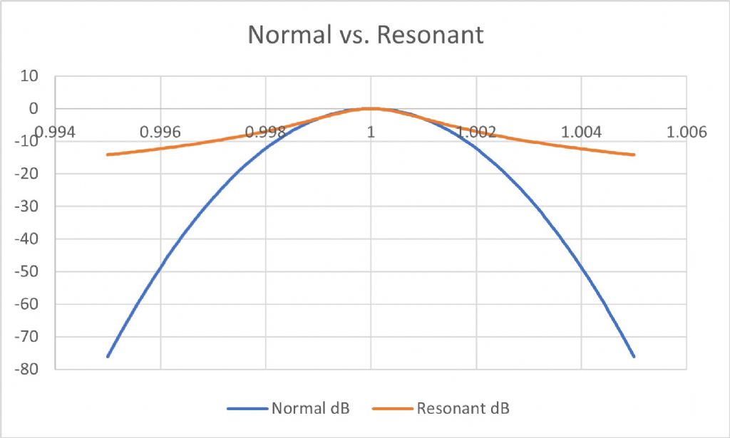
I thought it would be interesting to directly compare the normal distribution curve with a resonance curve according to the equation Dave quoted above.

In this picture the normal (blue) curve is plotted using Excel's normal distribution function normalised so the peak is unity. I've normalised the mean to unity and the standard deviation to the value that Dave measured divided by his period, to give 0.001194. I've plotted the vertical axis in dB to make it easy to compare the 3dB points. I wasn't quite sure how to render the vertical probability axis in dB since it doesn't really have a meaning but I chose 20*log10 to match what I did with the resonance formula. The resonance curve (orange) used the same centre frequency of 1Hz and I twiddled the Q to to get the -3dB points to match the normal curve, which needed a Q of ~500.

What's obvious is that though the curves are similar around the peak they diverge hugely as one moves away, by 10s of dB.

It seems to me that the period error must depend on the Q, obviously, but also on the "noisiness" of the whole oscillator, and the amplitude of the oscillation which the noise is perturbing. Those factors are captured in the equation I posted. Clock B is a nice example – the pendulum has a rather low Q compared to most regulators, but it swings with about 4 – 6x the amplitude, the drive torque is very accurately controlled with a remontoire, the escapement minimises frictional variation of force, the whole thing is extremely massive and (for the critical tests) was mounted on a masonry column embedded in boulder clay; and finally the pendulum is temperature and barometrically compensated.

I think Dave's distribution looks very gaussian (normal) and is actually a very useful measure though not of Q! It tells us I think that the systematic variations are pretty small and most of the fluctuations are random, though they could be due either to the oscillator or the measurement system.

[SillyOldDufferModerator @sillyoldduffer]

Posted by John Haine on 18/08/2023 11:05:14:

I thought it would be interesting to directly compare the normal distribution curve with a resonance curve according to the equation Dave quoted above.

In this picture the normal (blue) curve is plotted using Excel's normal distribution function normalised so the peak is unity. I've normalised the mean to unity and the standard deviation to the value that Dave measured divided by his period, to give 0.001194. I've plotted the vertical axis in dB to make it easy to compare the 3dB points. I wasn't quite sure how to render the vertical probability axis in dB since it doesn't really have a meaning but I chose 20*log10 to match what I did with the resonance formula. The resonance curve (orange) used the same centre frequency of 1Hz and I twiddled the Q to to get the -3dB points to match the normal curve, which needed a Q of ~500.

What's obvious is that though the curves are similar around the peak they diverge hugely as one moves away, by 10s of dB.

It seems to me that the period error must depend on the Q, obviously, but also on the "noisiness" of the whole oscillator, and the amplitude of the oscillation which the noise is perturbing. Those factors are captured in the equation I posted. Clock B is a nice example – the pendulum has a rather low Q compared to most regulators, but it swings with about 4 – 6x the amplitude, the drive torque is very accurately controlled with a remontoire, the escapement minimises frictional variation of force, the whole thing is extremely massive and (for the critical tests) was mounted on a masonry column embedded in boulder clay; and finally the pendulum is temperature and barometrically compensated.

I think Dave's distribution looks very gaussian (normal) and is actually a very useful measure though not of Q! It tells us I think that the systematic variations are pretty small and most of the fluctuations are random, though they could be due either to the oscillator or the measurement system.

No point in denying it – I'm worried, and have been since John emailed a couple of his papers to me last week . Not quite convinced myself yet I'm wrong about Q but I trust John's judgement in this area. So I spent this afternoon bashing my brains in hope of understanding it!

Doesn't prove anything but I produced these similar graphs, also comparing normal and resonant curves:

First up is my pendulum's frequency distribution.

Second is my pendulum's frequency distribution fitted to a normal distribution. The match is good suggesting my pendulum is producing normally distributed periods.

Third is a resonant curve generated from this formula found under 'Universal Resonance Curve' in Wikipedia's Resonance article:

ω is the natural resonant frequency
Ω is the drive frequency
Γ is the decay factor

Damping the third curve with a decay factor of 0.1 produces a curve similar to the actual pendulum distribution

Fourth graph is the resonance curve generated with a lighter decay factor. As expected it produces a much sharper curve.

No wonder I'm confused!

Dave

[duncan webster 1Participant @duncanwebster1]

Stepping gingerly as I'm not at all sure what I'm talking about, Dave's third and 4th curves relate to a resonant system being driven at a range of frequencies above and below the resonance. A pendulum is driven at its resonant frequency, or at say 1/15th for a Synchronome, or not at all when doing a run down test. I can't help feeling that these are 2 different scenarios. My pendulum keeps noticeable swinging for quite a long time if I turn the power off, can't exactly remember, but tens of minutes, does a inductor/capacitor manage this?

If I had a pendulum which was perfect in every way apart from a bit of damping and I let it run down, the frequency would very gradually increase as the amplitude decayed, but it wouldn't have a normal distribution.

[SillyOldDufferModerator @sillyoldduffer]

Posted by duncan webster on 18/08/2023 18:20:58:

… My pendulum keeps noticeable swinging for quite a long time if I turn the power off, can't exactly remember, but tens of minutes, does a inductor/capacitor manage this?

…

An LC circuit of the same Q and resonant frequency as a pendulum would take the same number of cycles to decay and hence the same time.

The decay formula is :

However LC circuits usually oscillate at much higher frequencies than pendula, so the number of cycles needed for an LC resonator to decay to the same level occur much faster, An oscillator of Q=10000 at 10MHz decays 10 million times faster than one of Q=10000 oscillating at 1 Hz.

Dave

[Michael GilliganParticipant @michaelgilligan61133]

Posted by SillyOldDuffer on 18/08/2023 17:44:37:

.

[…]

Damping the third curve with a decay factor of 0.1 produces a curve similar to the actual pendulum distribution

Fourth graph is the resonance curve generated with a lighter decay factor. As expected it produces a much sharper curve.

No wonder I'm confused!

Dave

 

.

With the greatest respect and empathy, Dave … I think even a damping factor of 0.01 [your fourth graph] would be appallingly high for a pendulum.

MichaelG.

.

Edit: __ in the case for the prosecution, I present this [found after I posted] well-documented, and easily replicated, experiment:  https://arxiv.org/pdf/2002.03796.pdf

Edited By Michael Gilligan on 18/08/2023 20:32:22

[John HaineParticipant @johnhaine32865]

Posted by duncan webster on 18/08/2023 18:20:58:

…..

If I had a pendulum which was perfect in every way apart from a bit of damping and I let it run down, the frequency would very gradually increase as the amplitude decayed, but it wouldn't have a normal distribution.

The period would decrease very slightly, but the cycle-to-cycle random variation would be very small unless there was a lot of noise affecting it (for example support vibration).

[Michael GilliganParticipant @michaelgilligan61133]

… For appallingly, please read rather

MichaelG.

[Martin KyteParticipant @martinkyte99762]

Not sure about the use of the general resonance formula as applied to an intermittently driven oscillator. ?

regards Martin

[SillyOldDufferModerator @sillyoldduffer]

Posted by Michael Gilligan on 18/08/2023 20:02:56:

Posted by SillyOldDuffer on 18/08/2023 17:44:37:

.

[…]

Damping the third curve with a decay factor of 0.1 produces a curve similar to the actual pendulum distribution

Fourth graph is the resonance curve generated with a lighter decay factor. As expected it produces a much sharper curve.

No wonder I'm confused!

Dave

.

With the greatest respect and empathy, Dave … I think even a damping factor of 0.01 [your fourth graph] would be appallingly high for a pendulum.

MichaelG.

.

…

Oh dear, a major breakdown of communications! No wonder – it's getting complicated,

My Graphs 3 and 4 are examples illustrating how the shape of a universal resonance curve depends on the damping factor. They're a response to John's post in which he compares a normal distribution curve to a resonant curve and suggests the curves move away from each other. I'm pointing out by example that the shape of a resonance curve can be made to look like a normal distribution by tweaking the decay factor. I said I don't believe it proves anything!

This part of the discussion relates to a serious criticism John is making of the way I calculate Q-factor using what I believe to be the valid bandwidth method. Serious because I'm an amateur poking around in the dark, whilst this is John's area of expertise and he can do the maths! At the moment I'm in the unhappy position of not understanding my own work or understanding why John thinks I've got it wrong.

My efforts this afternoon have shown my pendulum's frequency distribution is close to a normal distribution and that I can synthesise a resonance curve to take much the same shape. I'm no nearer proving to my own satisfaction that the way I calculate Q is right or wrong. Sadly, when an expert tells an amateur he's messed up, the expert is usually right…

Dave

[SillyOldDufferModerator @sillyoldduffer]

Posted by S K on 18/08/2023 01:15:27:

If I estimate your "half power bandwidth" to be 2 times your standard deviation (that's the number I have, anyway), then after rounding the numbers for simplicity, I get Q=1/(2*0.001)=500. How do you get over 20,000? What numbers do you have?

Also, you expressed concern about how your cumulative time error had wandered. This is due in large part to the accumulation of many small random errors in a classic random walk. If those small errors are 250 times lower (i.e., S.D. = 4us vs. 1ms), then the cumulative deviations should, in an typical run, also be 250 times lower. So yes, you do want as low a standard deviation as you can get.

…

An interesting development this afternoon! I found a code error. The standard deviation of my data isn't about 1mS, it's 0.037 milliseconds, which by SK's method above gives my pendulum Q=13500.

Sorry about that, my fault.

Assuming the data and method I'm using is correct, which has been strongly challenged by John, the 3db bandwidth of my pendulum is about 0.044 milliseconds, period 0.937357s.

Dave

[Michael GilliganParticipant @michaelgilligan61133]

Posted by SillyOldDuffer on 18/08/2023 21:59:10:
.

[…]

Oh dear, a major breakdown of communications! No wonder – it's getting complicated,

[…]

.

mea culpa …

but I would still recommend the brief paper that I linked.

MichaelG.

[Author]

Posts