JoNo’s Pendulum

[SillyOldDufferModerator @sillyoldduffer]

Posted by Michael Gilligan on 01/09/2023 21:34:21:

I am very rusty on this stuff, Jo … but I think you might want to use the natural logarithm:

…

MichaelG.

Not only am I rusty, but I was never smart in the first place! And my maths is dreadful. However, I'm happy to my have my thoughts marked out of ten. Could be embarrassing!

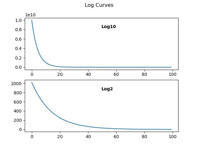
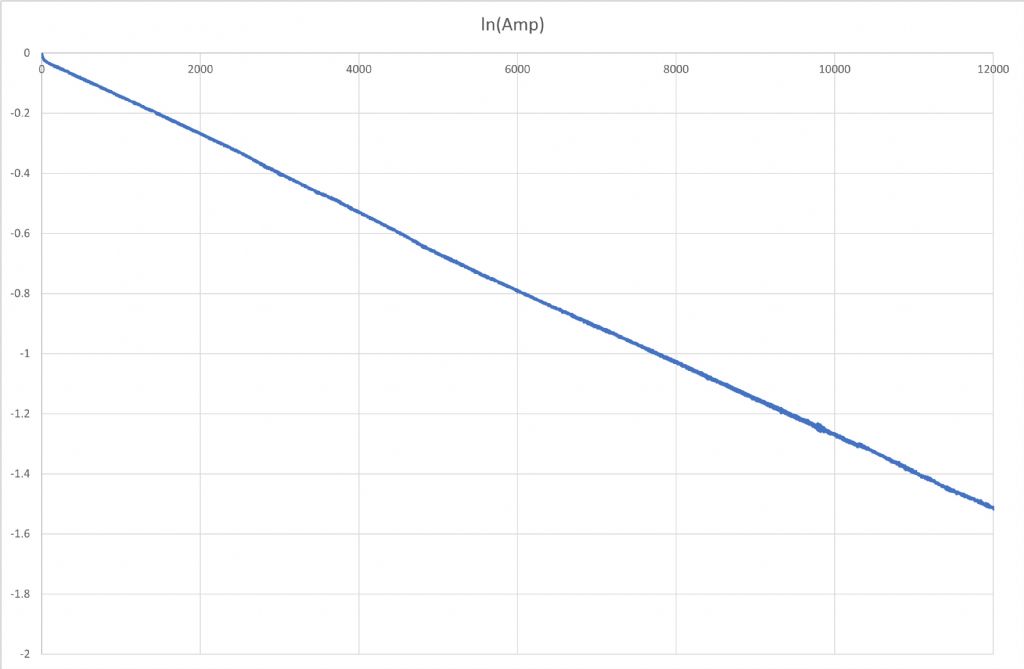
As I understand it, at this stage, the base of the logarithm doesn't matter. The shape of a logarithmic curve on a graph is representative of exponential decay, which is typical of energy being lost from a closed system. Joe's graph looks to have a curve characteristic of exponential decay, but we don't know what the exponent is.

Examples of exponential curves:

Point here is that Log Base 10 and Log Base 2 have the same basic shape, as does Joe's curve, except his could be log base 1.2 or something else. An exponential curve is one where a power is present in the equation that describes the curve. Powers less than 1 are roots. (√4 is 4 to the power 0.5)

If taking the log of a graphed curve tends to straighten it, then that's evidence the curve is exponential.

Many phenomena result in a straight-line graph. Many others produce curves and this class includes energy loss. A generator or chuck running down when power to the motor is cut, a bouncing ball, pressure falling in a emptying water-tank, mechanical oscillators overcoming friction, or electronic oscillators overcoming electrical resistance all produce exponential decay curves.

After a ball is dropped from a height it rebounds less and less on each bounce. If the rebound height is graphed per bounce, the curve will be found to decay exponentially. The energy loss on each bounce is non-linear. The value of the exponent depends on the mechanical nature of the floor and ball, and air resistance and can be calculated in various ways, such the least squares method.

To my mind knowing the exponent's value isn't all that useful, because for pendulista purposes it provides much the same information as Q. However, it's important to ensure that a pendulum's decay curve really is exponential because the Q calculation depends on it! I'd bet the farm that Joe's curve is exponential, but think it's a step too far to assume that's proof of aerodynamic resistance. Even though aerodynamic resistance is highly likely to be a major player. Fanning air is a major cause of energy loss in a pendulum, even if the bob is aerodynamically efficient.

Dave

[Michael GilliganParticipant @michaelgilligan61133]

That all looks fine to me [as far as it goes], Dave

But John did mention ‘straight line’ earlier … which is what I was picking-up on

Have a look at the page I linked last night: **LINK**

https://serc.carleton.edu/sp/library/teachingwdata/graphsexponential.html

and click on the first two of the three big yellow pictures to enlarge them.

That’s what a straight line should look like 

MichaelG.

Edited By Michael Gilligan on 02/09/2023 12:12:30

[duncan webster 1Participant @duncanwebster1]

I think my maths is a bit better than SOD's, but still not that good. However, I reckon the exponent is – 1/Q, or a multiple of it. It is analogous to the RC value in capacitor discharging through a resistor voltage decay. 

Edited By duncan webster on 02/09/2023 12:34:50

Edited By duncan webster on 02/09/2023 12:37:39

[Joseph Noci 1Participant @josephnoci1]

Its been an interesting day and last night…

Yesterday I replaced the V lateral pivots with pin on flats. After that the Q had dropped from around 12000 to 8000. I found issues with the knife edge alignment, and carefully adjusted that and di Q runs till the adjustment was at peak – Q done only at 61% (xPix2). This ended up at Q = 10000 average – still down on my 12500 achieved previously.

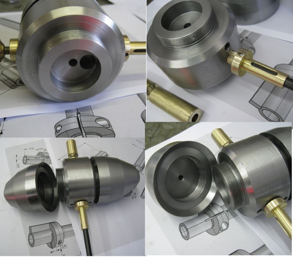
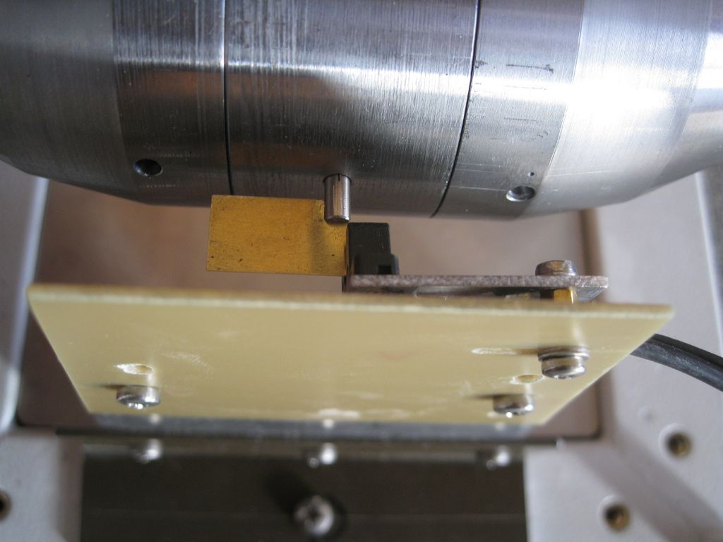
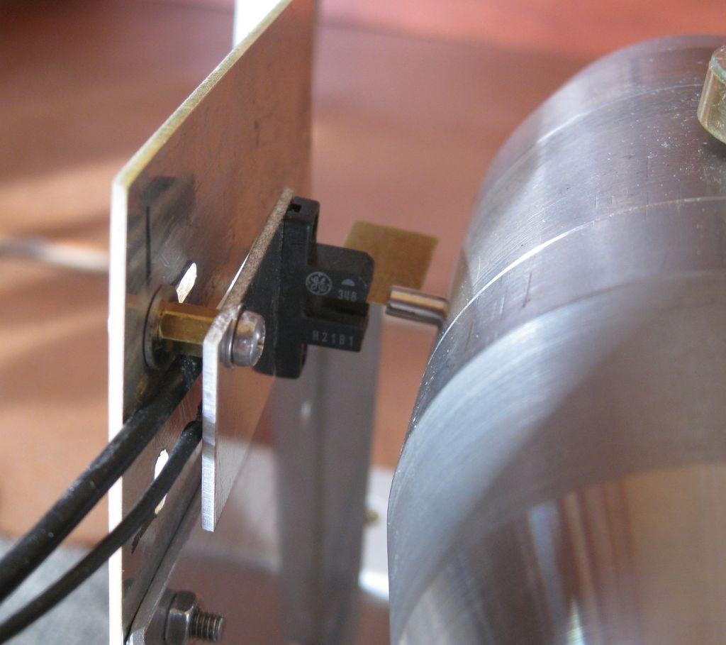
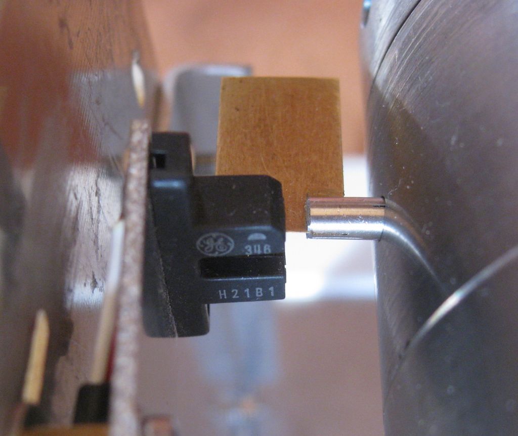
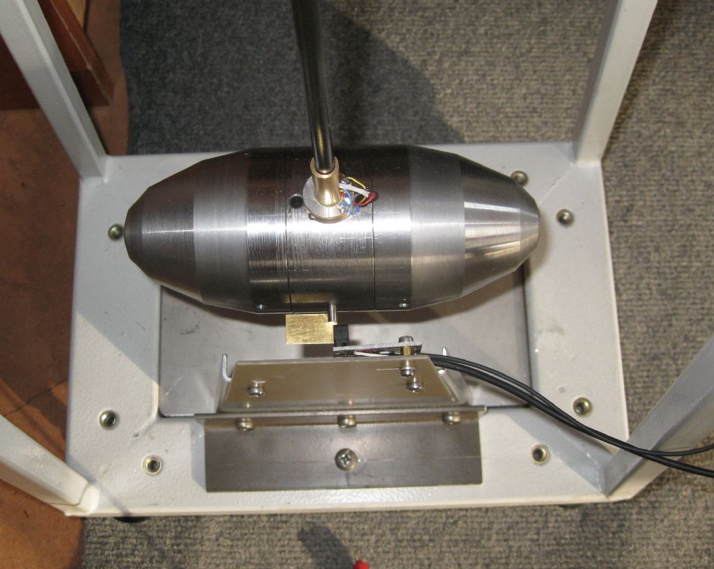
However, what I also did during the V pivot replacement was add the Opto interrupter and accompanying vane on the pendulum. The vane is a long vane – 20mm x 10mm, and starts at the opto slot at BDC, and then covers the slot completely for 1 half swing, so I get a 0.5Hz square wave out of the opto,

So…. I removed the vane and opto and did a run again – Q=12600! Did another, Q=12400…

Put the vane and opto back – made SURE there is no rubbing or touching, Q=10100 …

Removed the opto and the mounting plate and did another run – Q=11000…

And last, remove the vane as well, again, – Q=12550.

The aerodynamic effects of the Bob play a massive role on Q! Just that little vane, brass shim stock, costs 1000 in Q.

I must rethink the mechanics on the vane completely.

I tried using the zero crossing on me Angle sensor, but that gives me a few 10's of us jitter, which I would like to avoid.

I also have the bob adjuster protrude below the bob, a 20mm OD x 30mm long 'nut' . Now the bob position is almost on the sweet spot, I can adjust the rate with just the two top adjuster nuts, top near the pivot, so I will cut that bob nut flush with the bottom of the bob.

The nuts is seen in the lower left photo below, sticking out away from the rod.

I think we underestimate the effects of bob shape and bits that stick out on the aerodynamic result.

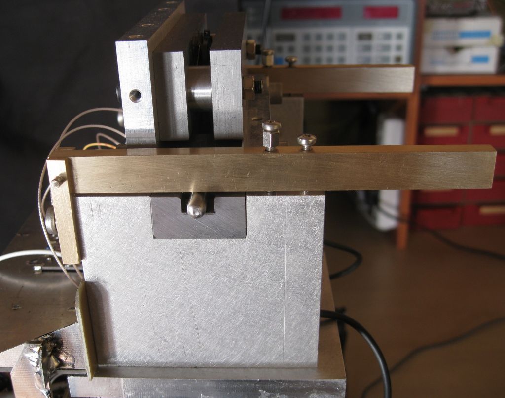
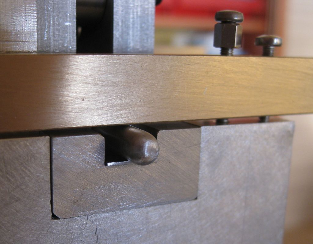
The new lateral pivots:

The brass bar can be screwed down hard on the pin, or it can be left floating on the pin, or it can be lifted so the pivot pin is free

The brass shim vane, center picture, almost in the opto

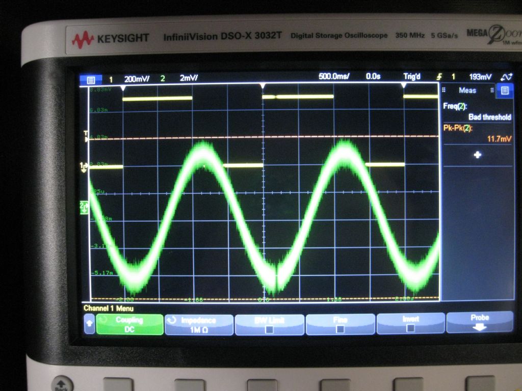
John asked I do a run-down and let it sit , logging data – I am still logging, but after 6 hours, the pendulum is still swinging – 117mv PP ( scope probes are X10) The angle sensor gives 2V PP for a 2deg swing, so this residual of 117mv is around 117millidegrees PP!

Walking about 3meters from the pendulum, 8 steps in 5sec, par to the pendulum, and the swing increases to 134mv..

Pendulum research in a town is difficult..

[S KParticipant @sk20060]

Posted by Joseph Noci 1 on 02/09/2023 11:48:37:

Unfortunately its not that simple – The knife riding in the curve is intentional as the capacitive angle sensor vane has to rotate around the pendulum pivot point, which is the knife contact edge. The sensor registers and van movement, which in my case must only be rotation around the pivot. Any movement of the knife on its ledge inthe swing direction is therefore a movement of the vane, indiscernible from movement due to rotation, so it registers and offset, ie, the angle sensor peak to peak measurement remains a constant, but the midpoint is offset by the amount the knife is moved.

So the curve is an attempt to avoid adjustment or calibration. I suppose calibration – subtracting an offset, or perhaps an offset and higher-order figures, etc., from the data – would be excessively problematic?

My concern about round anvils is that they are pseudo-flat: neither with a sharp enough curve to accurately position the knives in one fixed place, nor flat enough to avoid skewness.

I also really don't like the "scratch" method, mentioned above, that seeks to keep the knives in position – that's begging for a lot of extra friction. But fine vertical scratches or marks for the proper position, and the use of a loupe, should allow positioning the knife edges with quite good accuracy.

My understanding is that the big downside of flat knife rests (whether knife on flat or flat on knife) is that environmental disturbances can cause the pendulum to "hop" minutely, and eventually walk right off the edge. I never saw any evidence of that myself (and I live in a geologically-active region), but my knife-edge pendulum was never intended to run for months or years, and indeed most of the time it was not even rocking. Nevertheless, the fear of that led me to switch to spring hinges for my current effort.

[S KParticipant @sk20060]

Posted by Joseph Noci 1 on 02/09/2023 17:29:54:

The aerodynamic effects of the Bob play a massive role on Q! Just that little vane, brass shim stock, costs 1000 in Q.

You aren't alone. I recently read the old articles by Bateman on his clock. He reported similar drops in Q from such small add-ons. Really, every little nut and screw, etc., needs to be optimized for aerodynamics. That includes the surrounding apparatus that is near the pendulum, such as the opto, etc., that influences the air movement around the pendulum.

Until you are operating in a vacuum, you might as well just figure that, as far as Q is concerned, everything is about aerodynamics unless you are outright scornful of any other frictional sources such as the hinge.

 

Edited By S K on 02/09/2023 18:13:58

[Clive SteerParticipant @clivesteer55943]

To investigate the aerodynamics of a particular pendulum rod and bob weight design I would keep the Q low by maintaining the desired shape of the bob but reduce its weight. Reduced Q provides a faster loss of amplitude enabling any aerodynamic tweaks to be evaluated more rapidly.

Interference drag is a problem in aircraft where the wing meets the fuselage and root fairings are a common solution. In this instance this is where the pendulum rod meets the bob and a fairing may be beneficial.

CS

[Joseph Noci 1Participant @josephnoci1]

Clive:

It is rather complex when trying to scale these things though. As an Aeronautical Eng I am familiar with the art and techniques employed on these subjects. Often though, modelling could be turned into prototypes and evaluated in the wind tunnel – Pendulums are another story! In Namibia, where I moved to after retirement, for South Africa, there is no such industry at all – I am the ONLY ' MEW modeler' in the country..I do have some reasonably good Aerodynamics modelling SW, but it can be in error by large amounts at these low Reynolds numbers…

I fully expected the vane to have an effect, but not such a large one. The shape of the bob was an 'educated' evolution from a model I tested at higher Rnumbers – 2000 and up.! Basically reducing R to see where reduction/increase in drag and laminar flows became severely non-linear. Since the use of trips on leading edges holds essentially true at all Reynolds numbers ( except at supersonic speeds..), the shape of the bob was born out of that model, with the cone's edges as trips. The pendulum has turned out to be very sensitive and the Q not bad, so maybe that was a sound solution, and maybe that is confirmed by how badly the Q is affected when I mess with that shape by adding vanes. I recall a few programs on UAV's I developed where we attached Vane angle of attack probes on the aircraft nose section, one for side slip and one for AoA – the placement was crucial – to the aircrafts aerodynamics, but majorly so to the probe! Fairings were the order of the day on those probes.

Also, my environment makes it difficult to evaluate small effects – For parts of the day we have 7-10ms wind speeds that buffet the studies large glass windows and doors, and the Atlantic with big waves 50meters from the house.

Last night I turned of the pendulum and let it coast down – for 7 hours. This morning the scope logged a 82mV PP swing on the pendulum angle sensor ( around 80millidegrees) and that was almost constant for the last 3 hours of logging. It does not stop – and the wind was below 3m/s for the evening.

I would like to machine the bob into a smooth surface and see what that does to Q, but there is no coming back from that and I don't have the motivation to make a new bob..

 

Edited By Joseph Noci 1 on 03/09/2023 07:38:18

[Joseph Noci 1Participant @josephnoci1]

Posted by S K on 02/09/2023 17:58:21:

So the curve is an attempt to avoid adjustment or calibration. I suppose calibration – subtracting an offset, or perhaps an offset and higher-order figures, etc., from the data – would be excessively problematic?

Not really – It may have got lost in my explanation of how the drive to the pendulum works-

I use the sinus from the angle sensor to feed the drive coils, with a 90deg phase shift. That 90deg sinus is amplitude controlled to control the bob amplitude. The control loop uses the peak value of the angle sensor sinusoid to determine the amplitude , against an accurate temp stable band gap DC reference voltage. So there is no software in the loop at all – purely an analogue electronic control loop, If the angle sensor has an offset, in my electronics this is seen as a change in PP value – the sinus cannot be AC coupled since other effects take over at such low frequencies (0.5Hz). The change in PP value, from a constant offset, is anew amplitude control value, which is incorrect.

I am busy making a new peak detector, or rather an RMS= to DC converter, that is thermistor based – The sinusoid heats a thermistor in a bridge, with the control loop heating the bridges thermistor mate to balance the bridge – the voltage applying to the latter is also used to control the amplitude of the voltage applied to the pendulum coil.

The time constant on the thermal process is some 10's of seconds, and that works well. The DC offset I balance out in the thermal loop, so it should work well.

It is gilding the Lily, since once the pendulum is set up, and the angle sensor vane it set so there is no offset, the system works fine, and if I do not move the pendulum around, all stays well.

I want the software to only do environmental correction at the end – no time monitoring or control at all – even the vane and opto will be removed in the end. If I can keep amplitude truly constant, I only have to adjust the bob to get 0.5Hz, and let software fix environmental changes.

[SillyOldDufferModerator @sillyoldduffer]

Posted by Joseph Noci 1 on 03/09/2023 07:32:21:

…

I fully expected the vane to have an effect, but not such a large one. …

Also, my environment makes it difficult to evaluate small effects – For parts of the day we have 7-10ms wind speeds that buffet the studies large glass windows and doors, and the Atlantic with big waves 50meters from the house.

Last night I turned of the pendulum and let it coast down – for 7 hours. This morning the scope logged a 82mV PP swing on the pendulum angle sensor ( around 80millidegrees) and that was almost constant for the last 3 hours of logging. It does not stop – and the wind was below 3m/s for the evening.

…

I too was surprised by what the vane did to Q, but on second thoughts maybe not. Q-factor is a very sensitive measure of a high-performance pendulum, and small spoilers show up vividly when Q is high. Measuring Q is valuable because there may be an easy answer, in this case do something about the vane! A better answer, but harder to do, is to remove the air.

That pendulums start swinging from a stop on their own is mentioned in the literature. Again, the better a pendulum is, the more likely it is to self-start. It happens when a pendulum has low friction and is sharply tuned to a frequency. Being sharply tuned means that external energy impulses cause the pendulum to oscillate. External energy must also affect a powered pendulum, causing amplitude and frequency to vary ever so slightly,

I suspect a heavy bob, swinging on a stand, is detecting Joe's home is moving. Locating the clock above ground level makes it more sensitive because the walls amplify movement by acting as levers.

Not unusual for buildings to move: some skyscrapers sway several inches off true in high winds. Smaller buildings also move due to heating and cooling, people moving about inside, vehicles moving outside, and the geology underneath. Living on the South Atlantic sea-board means Joe has millions of tons of water moving about on his door step. Be more surprising if the pendulum didn't pick anything up,

Dave

 

 

 

Edited By SillyOldDuffer on 03/09/2023 10:19:01

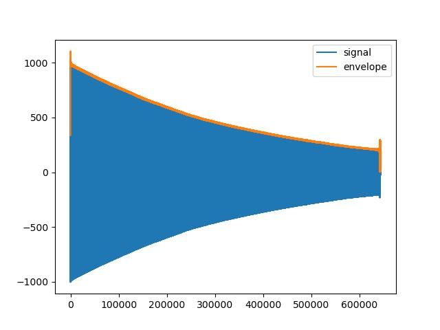
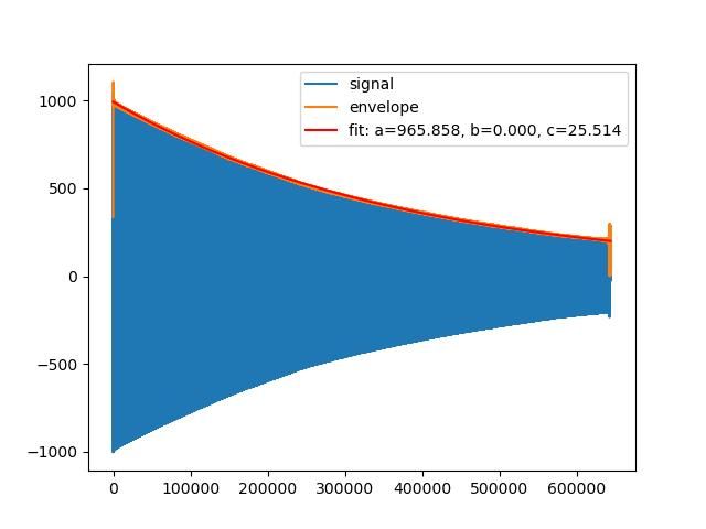
[SillyOldDufferModerator @sillyoldduffer]

Had a go at Joe's amplitude data in hope of identifying his decay curve's values. Mixed success, first problem is to extract the envelope of the signal, which looks good.

In the graph below, Joe's signal, composed of sinusoidal amplitude readings. is in blue, whilst the envelope retrieved from the signal is in orange.

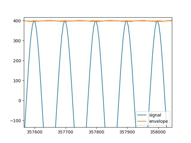
I expected the orange curve to simply connect the peaks of Joe's data, and it doesn't. Zooming in on the orange line shows it also appears to carry a signal:

Not sure why. Possibly to do with Joe's 20mS sample rate, or a mathematical artefact. Or maybe it's a real-world pendulum imperfection. Dunno.

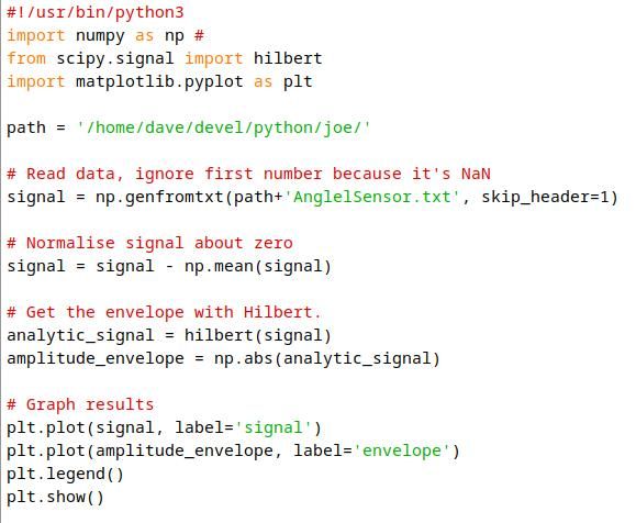
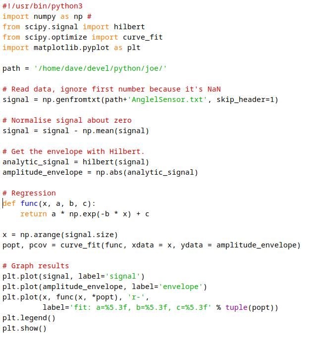
Code so far:

Next step is to fit a curve to the envelope and reveal its parameters. First attempt wrong, now looking at scipy.optimise.curve_fit. If only I understood it!

Dave

[John HaineParticipant @johnhaine32865]

I've also had a go at the data that Joe was kind enough to share. He provided a file of essentially voltage samples from his angle sensor. These have a pronounced DC offset on them, larger than the negative peak, so I subtracted the mean value of all the readings from each to get a symmetrical waveform. There was also quite a lot of noise which made it hard to reliably find the peak so I did some crude filtering by replacing each value with the average of five (the sample plus the 2 before and the 2 after); then took the absolute value to include the negative peaks. Then extracted the peak readings using the Excel filter function. Normalised each sample to the value of the first and took the natural log to get this (for the first 12,000) seconds).

That looks a pretty straight line to me! It reaches a value of -1 at 7800 seconds in, so the time constant is 7800 seconds. This is equal to 2Q/w where w is the angular resonant frequency, in this case 2pi x 0.5 = pi. Then

Q = pi x 7800/2 = 12,250, very much in the ballpark Joes was measuring.

I think the reason Joe was getting a strange decay shape was that he took the log of the peaks of the raw data which included the dc offset.

Really awkward using Excel for this because there's so much data!  Would be better to use something like R-Studio but I'm not sure it has all the functions needed.

 

Edited By John Haine on 03/09/2023 15:43:58

[Michael GilliganParticipant @michaelgilligan61133]

Nice one, John

MichaelG.

[John HaineParticipant @johnhaine32865]

One thing to add is that this seems to show that the loss mechanism is nearly entirely simple viscous loss.

[Michael GilliganParticipant @michaelgilligan61133]

Get that vacuum pump going, Jo

MichaelG.

[Joseph Noci 1Participant @josephnoci1]

Posted by John Haine on 03/09/2023 15:42:05:

I've also had a go at the data that Joe was kind enough to share. He provided a file of essentially voltage samples from his angle sensor. These have a pronounced DC offset on them, larger than the negative peak, so I subtracted the mean value of all the readings from each to get a symmetrical waveform. There was also quite a lot of noise which made it hard to reliably find the peak so I did some crude filtering by replacing each value with the average of five (the sample plus the 2 before and the 2 after); then took the absolute value to include the negative peaks. Then extracted the peak readings using the Excel filter function. Normalised each sample to the value of the first and took the natural log to get this (for the first 12,000) seconds).

That looks a pretty straight line to me! It reaches a value of -1 at 7800 seconds in, so the time constant is 7800 seconds. This is equal to 2Q/w where w is the angular resonant frequency, in this case 2pi x 0.5 = pi. Then

Q = pi x 7800/2 = 12,250, very much in the ballpark Joes was measuring.

I think the reason Joe was getting a strange decay shape was that he took the log of the peaks of the raw data which included the dc offset.

Really awkward using Excel for this because there's so much data! Would be better to use something like R-Studio but I'm not sure it has all the functions needed.

Edited By John Haine on 03/09/2023 15:43:58

John, that is excellent work. Thank You. I am pleased the device behaves to some norm..

The DC offset on the sine is there because I am presently using the CPU's A/D to sample the waveform, and the A/D only accepts +ve values. My peak to peak is normally around 2v, so I have an offset a bit more than 1v. I wrote a Python bit of code that extracts the peak values of the +ve and -ve and puts them in a file. The fact that there is a DC offset there should no really affect the Log though? I need to try a little harder – I normalised those values but the Log is still not straight – I suspect because of the DC offset?

What sort of noise level are you finding on the data?

There are two issues related to the noise – the one is system noise – that from the op-amps, the wiring and the related noise on samples by the A/D – the A/D is processor bound, and its reference grounds are therefore shared somewhat with the CPU digital ground so there are always a few LSB's of inherent noise ( 12bits = 3v range).

The second source, and I think Dave found this 'ripple' on the peaks, is embedded in the amplitude control loop – the Peak detector I use to find peak swing is a simple op-amp/diode/cap peak detector and the value of the cap, which stores the peak, plays a major role here. Since the peaks are two seconds apart, the voltage on that cap droops before the next peak – I have 100uf in there, more creates loop instability. And there is a nice 3 to 5mv droop between peaks which feeds the VGA which controls the coil drive voltage, etc. The cap discharge R across it is 10megohm.

That needs some work – I am looking at a Thermal RMS-DC converter ( I wish one could still find the LT1088 !) – a simulation of the concept shows the thermal lag will overcome the droop, without compromising loop response time.

[SillyOldDufferModerator @sillyoldduffer]

Posted by SillyOldDuffer on 03/09/2023 14:25:11:

Had a go at Joe's amplitude data in hope of identifying his decay curve's values…

…

Next step is to fit a curve to the envelope and reveal its parameters. First attempt wrong, now looking at scipy.optimise.curve_fit. If only I understood it!

Dave

A result:

From y = a * np.exp(-b * x) + c

The parameters are: a = 9.65858457e+02, b = 2.66220695e-06, c = 2.55142704e+01

numpy,exp() documented here. Returns the exponent eᕁ, the inverse of natural log,

The code:

Dave

[John HaineParticipant @johnhaine32865]

"The fact that there is a DC offset there should no really affect the Log though?"

Very much so I'm afraid. An offset in an exponential, like exp(x+k) just results in a scaling:

exp(x+k) = exp(k) x exp(x)

Logs are different:

But log(x+k) = log(x) + log(1+k/x) (according to Wikipedia).

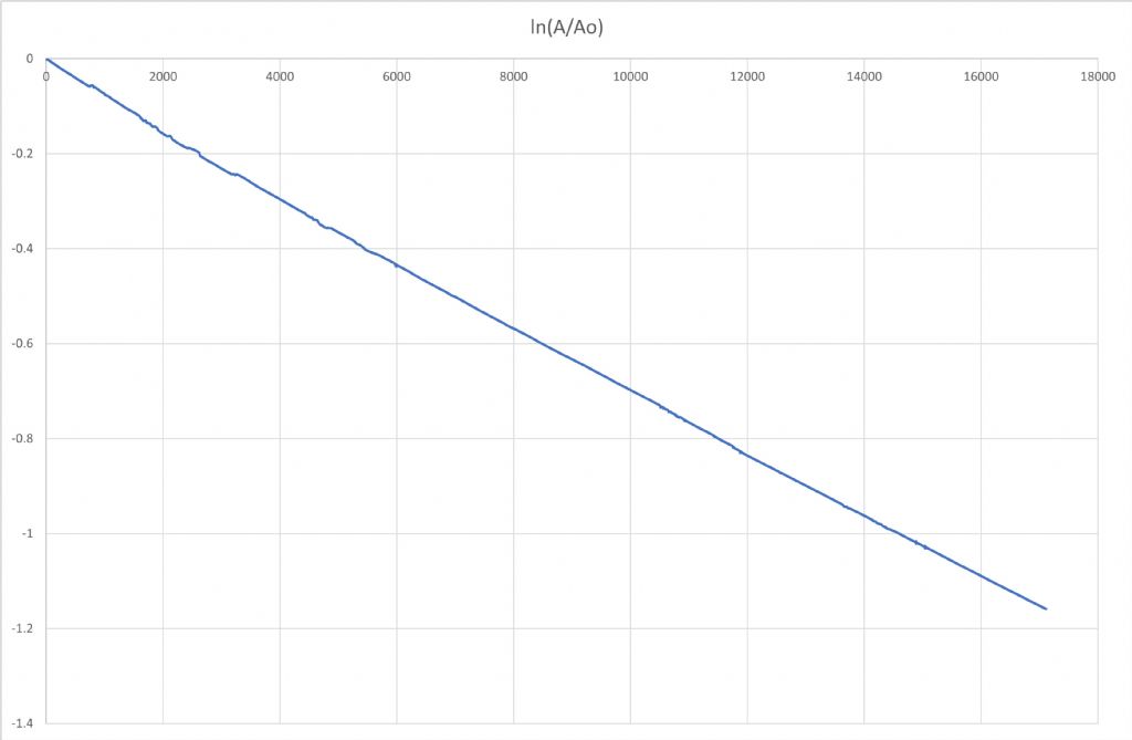
[John HaineParticipant @johnhaine32865]

I just thought I should repeat the rundown test on my own new pendulum so it has been coasting down since 1pm.

Again the log of normalised amplitude is -1 at 14612s in, so the same formula gives a Q of ~23,000, roughly what I got before.

Edited By John Haine on 03/09/2023 18:01:45

Edited By John Haine on 03/09/2023 18:23:13

[Joseph Noci 1Participant @josephnoci1]

Posted by John Haine on 03/09/2023 18:00:05:

I just thought I should repeat the rundown test on my own new pendulum so it has been coasting down since 1pm.

Again the log of normalised amplitude is -1 at 14612s in, so the same formula gives a Q of ~23,000, roughly what I got before.

Edited By John Haine on 03/09/2023 18:01:45

Edited By John Haine on 03/09/2023 18:23:13

Twice mine – Mine obviously is lacking – what is your advice?

[S KParticipant @sk20060]

Posted by Joseph Noci 1 on 03/09/2023 19:41:07:

Twice mine – Mine obviously is lacking – what is your advice?

Get a tungsten bob. Seriously. Yours is not dense enough in comparison.

Edited By S K on 03/09/2023 21:04:04

[SillyOldDufferModerator @sillyoldduffer]

Posted by Joseph Noci 1 on 03/09/2023 19:41:07:

Posted by John Haine on 03/09/2023 18:00:05:

…

Twice mine – Mine obviously is lacking – what is your advice?

My first suspect is the stand, because it's an important part of the system:

• The uprights are tall and thin, with a hefty bob swinging below. The construction is undoubtedly strong, but how much does it flex? Any elasticity whatever in the frame absorbs energy and reduces Q.
• Although the base is good and heavy, the feet might wobble or be made of rubber, both of which will also absorb.

Try bouncing a laser pointer off a mirror placed on top so that any movement of the stand at the suspension is amplified at the distant dot. Might be interesting as well to measure Q with the stand stood on a soft rug rather than tiled floor.

Dave

[Michael GilliganParticipant @michaelgilligan61133]

Posted by SillyOldDuffer on 03/09/2023 21:01:22:

Posted by Joseph Noci 1 on 03/09/2023 19:41:07:

Posted by John Haine on 03/09/2023 18:00:05:

…

Twice mine – Mine obviously is lacking – what is your advice?

My first suspect is the stand, because it's an important part of the system:

 

.

As will be clearly demonstrated by the example of two pendulums mounted on a substantial beam gradually synchronising.

[ sorry, can’t remember whom to credit ]

MichaelG.

.

 … it was my hero:

https://physicsworld.com/a/the-secret-of-the-synchronized-pendulums/

Edited By Michael Gilligan on 03/09/2023 21:21:44

[duncan webster 1Participant @duncanwebster1]

Friend of mine bought a Pulsynetic, it wouldn't run at all when stood on his carpeted floor, buts works nicely when bolted to a brick wall

[Joseph Noci 1Participant @josephnoci1]

The last Q run now shows Q to be near to 14000. Q has been slowly increasing over the last 36hours of running – My setup is reasonably stable and consistent and I tend to trust the Q determination. I suspect the increase is all related to the knife pivot. The knife sits in the curve of the bearing inner race and I believe it is not always in the bottom of the curve after any mechanical work on the pendulum. The pendulum rocking motion plus gravity slowly lets the knife ride down to the lowest part of the curve and when there, there is no lateral force on the pendulum, which induces a lateral swing ( 90deg to the main swing..)

When the knife is at the bottom the Q is good. Comfortingly, I have found a modulation on the angle sensor voltage output which started with a 10sec period ( the peak to peak voltage of the 0.5hz sine swing varies by 3 or 4 mV at 10sec period) and the period increased to with the mV delta now almost being almost indiscernible as the knife beds in. This I believe reinforces the knife bedding concept.

The pendulum period is presently measured against my GPSDO 0.5hz output. I sat and fiddled with the pendulum adjuster weights till the delta remained fixed , ie , no drift, at that moment and used that as my baseline. I logged lots of data over a large number of hours and the pendulum shows very well the period variation with ambient conditions.

The ambient temp in the study does not change more than 2deg over 24hours and there seems little correlation between temp and period at this stage. The bob and the rod temp change by 1deg max over that period.

Humidity is reasonably stable in the study – variation during logging was from 44% to 45.5%, and there seems to be no correlation between humidity and period change.

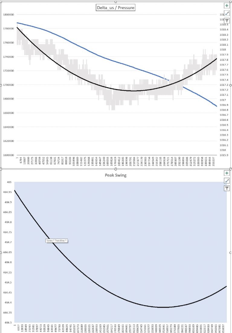
Pressure, on the other hand, seems to dominate.

The curves below:

Top chart , left scale, Blue curve = delta in us, over 5 hours horizontal scale. ( 2,000,000 us – 2sec period)

Top chart , right scale is pressure in millibar, max was 1018.4mb , min 1017.2mb

Bottom chart – the peak swing in millivolts ( or millidegrees) of the pendulum – It follows the pressure curve nicely, with a phase shift that is close to the current control loop response time.

This seems to show that the swing is increased as the pressure increases which 'sounds' correct – the bob is slowed as pressure rises so the swing reduces, and the system gain then increases to get the swing back up again. It makes sense, but I am not sure.

This curve is the output of the peak detector that is fed by the sine swing from the angle sensor – Intuitively I would have thought that curve should be flat – If the sine peak reduces the gain increases, driving the coil harder, the swing increases back to the setpoint, and the swing level is back to setpoint.

I am trying to extract the total control loop transfer function as that is key to the understanding I believe.

A further complication, due to lack of suitable components – the Voltage variable gain amplifier I use is a linear-in-dB device – the angle sensor output is peak detected and finally drives the voltage control input of the VGA – a 33mv change is a 3dB gain change. So the control is logarithmic and the resulting bottom curve is also log, etc –

I think there is great potential for the method of amplitude control, but there are too many unknowns for me and I am a bit lost!

[Author]

Posts